Prepare Data for GalfitS
Image Preparation
Overview
This section documents the imaging preparation pipeline in GalfitS. The process is designed to prepare astronomical images for further analysis through the following steps:
Sky Subtraction – Removing the background sky signal using a polynomial fit.
Image Cut and Mask Generation – Extracting a subimage around the target source and creating a corresponding mask.
Output Writing – Saving the processed cut image, mask image, and sigma image to a FITS file.
Step 1: Sky Subtraction
The first step is to subtract the sky background from your image. This is achieved with the sky_subtraction function from the galfits.images module. Here, a 3rd order polynomial is used to model the background, and sigma-clipped statistics are employed for image normalization and visualization.
Example code:
from galfits import images as IM
from astropy.io import fits
from astropy.stats import sigma_clipped_stats
import matplotlib.pyplot as plt
import gsutils  # assumed to be available for image normalization

# Define file name and load the image
fname = './data/tmass_{0}'.format(band)
img = IM.image(fname+'.fits', unit='cR')
hdu = fits.open(fname+'.fits')
header = hdu[0].header
data_org = hdu[0].data

# Define the output file for the sky-subtracted image
ss_imgname = './data/tmass_{0}_ssimg.fits'.format(band)

# Perform sky subtraction with a 3rd order polynomial
maskplus = img.sky_subtraction(polyfit=True, order=3, filepath=ss_imgname,
                               psfFWHM=3, nsigma=3.0, npixels=5,
                               max_grow_size=100, addgrow=0)

# Calculate sigma-clipped statistics for visualization
sky_mean, sky_median, sky_std = sigma_clipped_stats(data_org, sigma=3.0, maxiters=5)
immin = 1 * sky_std
immax = 5 * sky_std

# Visualize the original image, sky-subtracted image, and the subtracted sky
fig = plt.figure(figsize=(18,6))
ax1 = fig.add_subplot(131)
ax1.imshow(gsutils.normimg(data_org, immin, immax, sky=sky_median, frac=0.6),
           cmap='seismic', origin='lower', vmin=-1, vmax=1, interpolation='nearest')
ax2 = fig.add_subplot(132)
ax2.imshow(gsutils.normimg(data_org - img.data.data, immin, immax, sky=sky_median, frac=0.6),
           cmap='seismic', origin='lower', vmin=-1, vmax=1, interpolation='nearest')
ax3 = fig.add_subplot(133)
ax3.imshow(gsutils.normimg(img.data.data, immin, immax, frac=0.6),
           cmap='seismic', origin='lower', vmin=-1, vmax=1, interpolation='nearest')
plt.show()
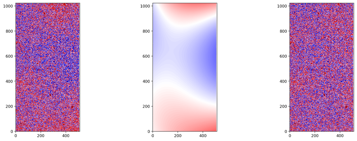
2MASS H-band image showing the results of sky subtraction.
Step 2: Image Cut and Mask Generation
Following sky subtraction, the next steps are to extract a cutout around the target source and to generate a mask to isolate the source. The functions used are:
img_cut: Cuts the image based on the source’s right ascension and declination.
generate_cutmask: Creates a source mask by detecting pixels above a threshold, optionally deblending overlapping sources.
Example code:
# Define cutout radius in arcseconds
cutr = 2.5  # unit: arcsec

# Extract the image cutout around the target (ra, dec)
imcut, cp = img.img_cut(ra, dec, cutr)
header = hdu[0].header

# Calculate the sigma image for the cutout
sigimg = img.cal_sigma_image(200, gain=1.)
img.cut_sigma_image = sigimg[cp[2]:cp[3], cp[0]:cp[1]]

# Generate the cut mask image using the specified parameters
img.cut_mask_image = img.generate_cutmask(psfFWHM, data=imcut,
                                           nsigma=2.0, npixels=150,
                                           nlevels=32, contrast=0.001,
                                           deblend=False, growmethod=True,
                                           max_grow_size=15, addgrow=addgrow)

# Write the cut images to a FITS file
outname = './cutimg/tmass_{0}_cut.fits'.format(band)
img.write_imcut(ra, dec, outname, header=header)

# Visualize the cutout with the mask overlay
fig = plt.figure(figsize=(8,8))
sky_mean, sky_median, sky_std = sigma_clipped_stats(imcut, sigma=3.0, maxiters=5)
sky_median = 0.0
immin = 5 * sky_std
immax = imcut.max()
frac = 0.4
plt.imshow(gsutils.normimg(imcut, immin, immax, sky=sky_median, frac=frac),
           cmap='seismic', origin='lower', vmin=-1, vmax=1, interpolation='nearest')
plt.imshow(mask0.astype(float), cmap='Blues', alpha=0.5 * mask0.astype(float),
           origin='lower', interpolation='nearest')
plt.savefig(resupath + '{0}_{1}_cutout.png'.format(tagname, band))
plt.show()
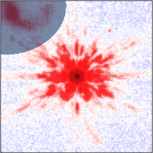
Example of an image cutout with an overlaid mask.
Functions Overview
Several key functions in the galfits.images module are utilized in this pipeline:
sky_subtraction(sdmask=None, polyfit=True, order=3, filepath=None, psfFWHM=1.5, nsigma=3.0, npixels=5, max_grow_size=100, addgrow=0, usemedian=False) Performs sky background subtraction using either a polynomial fit (default) or median subtraction. Parameters such as order, psfFWHM, and nsigma control the subtraction process.
img_cut(ra, dec, cutsize, cutposition=None, IFS=False, usemaxpix=False, sigma_clipped=True, referpix=None, zoomsize=100, spcorrection=[0.,0.]) Cuts the image around a specified celestial coordinate (ra, dec). Optional parameters allow for fine-tuning the cutout region.
generate_cutmask(psfFWHM, data=None, sdmask=None, nsigma=3.0, magnification=3., npixels=5, nlevels=32, contrast=0.001, deblend=False, sky_level=None, source_dia=0.5, max_grow_size=100, growmethod=True, nearbygrow=0, addgrow=0, left_source=True) Generates a mask for the cutout image by detecting sources above a given threshold. It supports various parameters for deblending and controlling the mask growth.
write_imcut(ra, dec, outputname, header=None, addpixsc=False, addmodel=False) Saves the processed image cutout along with the mask and sigma images to a FITS file. The output file includes all the relevant image components needed for subsequent modeling.
Conclusion
The image preparation module in GalfitS streamlines the process of preparing astronomical images by automating sky subtraction, image cutouts, and mask generation. This ensures that the data used in subsequent modeling are clean, well-calibrated, and precisely focused on the target sources.
Construct Empirical PSF
Overview
This section describes the process for constructing an empirical Point Spread Function (PSF) using the generate_PSFs function from the galfits.images module. The procedure comprises two main stages:
Selection of Real Point Sources: Identify and clean a catalog of candidate stars from the image. This involves source detection, optional cross-matching with the Gaia catalog, and several filtering steps (flux, geometric, isolation, and central pixel checks).
PSF Fitting: Perform PSF fitting on the cleaned sample of point sources. The fitting process optimizes the empirical PSF model, the source centers within their cutout boxes, and the flux normalizations.
Example Code
# read data
imgname = "./J003515.16+084859.9/ls10/170921_055634_g.fits"
outname = "./J003515.16+084859.9/ls10/psf/170921_055634_g_psf.fits"
with fits.open(imgname) as hdu:
    head = hdu[1].header
    data = hdu[1].data

# creating an image instance and generating epsf
img = IM.image(imgname, hdu=1, unit="cR")
sigmaimg = img.cal_sigma_image(expo, gain=gain, fac1=1., fac2=1.)  # expo & gain need to be set to real values

epsf = img.generate_PSFs(
    # Source detection parameters
    psfFWHM=1.7,
    data=data,
    nsigma=3.0,     # for detect_threshold
    npixels=50,     # for detect_sources

    # Real point source catalog construction
    sigmaimg=sigmaimg,
    crossmatch=True,
    starcord_list=None,   # input list of star coordinates: [[ra, dec], ...]
    fluxthreshould=0.,    # drop ultra-faint sources
    qt=0.1,               # axis ratio threshold for cleaning elongated sources
    sigfwhm=3,
    medianfwhm=11.5,
    size=81,
    isolate=0.3,
    central_tol=2,
    droppsf=[3,6,12,13],
    plot=True,
    figurepath='./',

    # PSF fitting parameters
    notfit=False,
    photutils_method=False,
    oversampling=1,
    a_TV=0,
    a_sky=0,
    learning_rate=2e-5,
    num_steps=80000,
    makestackpsf=False,
    filepaths=outname,
    verbose=True,
)
Selection of Real Point Sources
The generate_PSFs function first detects sources to build an initial raw catalog.
Because this catalog can include galaxies and artifacts, several filters are applied:
crossmatch=True: Cross-match candidates with Gaia DR3 stars; matching radius is \(1.5\times\mathrm{psfFWHM}\).starcord_list: Optional user-provided star coordinates to override auto-detected candidates.fluxthreshould: Remove very faint candidates below a fraction of the mean catalog flux.qt: Keep nearly round sources based on axis ratio.sigfwhmandmedianfwhm: Reject FWHM outliers (too broad or too narrow).sizeandisolate: Require clean neighborhoods inside a \(\mathrm{size}\times\mathrm{size}\) stamp.central_tol: Reject candidates with too many bad pixels near the source center.droppsf: Manually drop known problematic candidates by index.
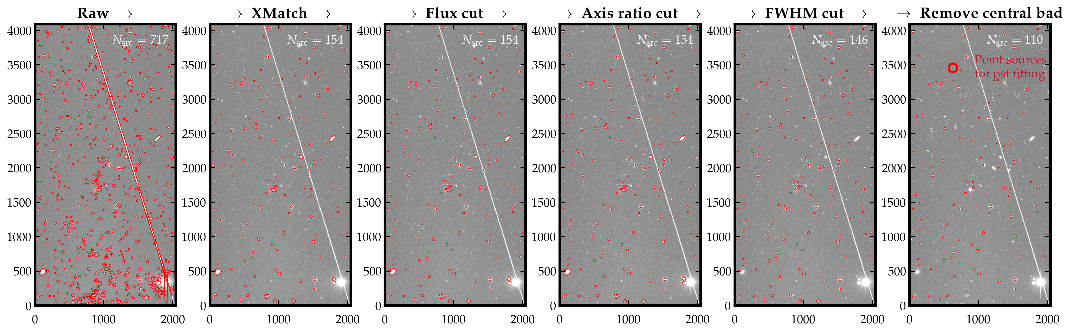
Fig. 1. Summary of the real point source catalog construction process.
PSF Fitting
After constructing a clean sample of point sources, the function proceeds to fit an empirical PSF. With notfit = False, the fitting process optimizes three main components:
Empirical PSF Model: The resulting PSF is a normalized $$text{size} times text{size}$$ image representing the combined information of all selected point sources.
Center Determination: The precise center of each point source within its box is determined.
Flux Normalization: Each source is assumed to be a scaled version of the PSF, and the algorithm optimizes the scaling factors.
The PSF fitting minimizes a loss function that compares the observed data with the PSF model, incorporating regularization terms (controlled by a_TV and a_sky) to penalize overly sharp features or background variations. The process is iterative, controlled by parameters such as:
learning_rate: Determines the convergence speed.
num_steps: The total number of fitting iterations.
oversampling: Adjusts the spatial resolution of the PSF if a value greater than 1 is provided.
photutils_method: Option to use the photutils fitting method; here, the built-in GalfitS method is used (set to False).
The final empirical PSF model, along with the derived source centers and flux normalizations, is saved to the output file specified by filepaths.
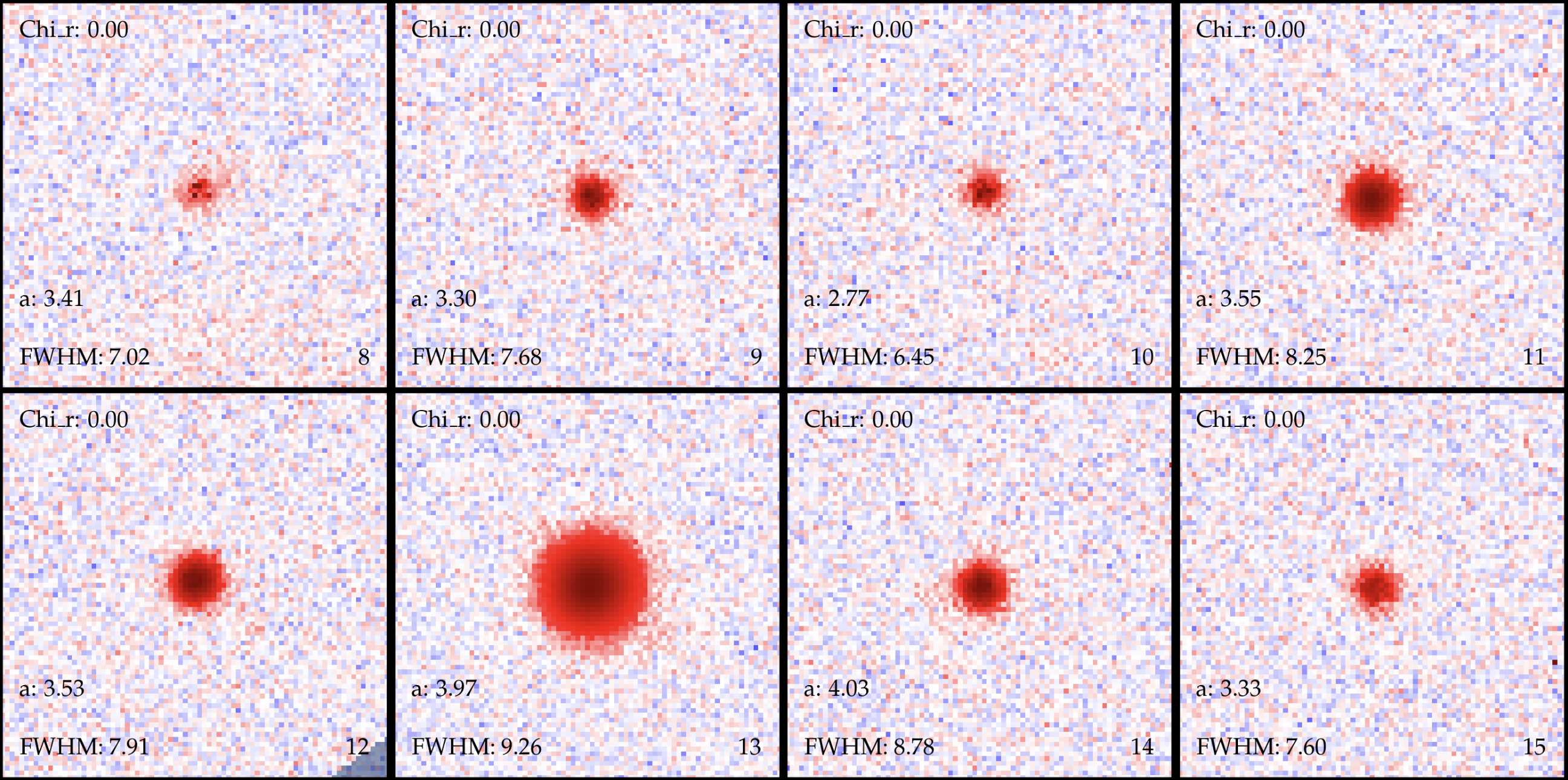
Fig. 2. Selected star candidates used for PSF fitting.
Conclusion
The generate_PSFs function seamlessly integrates source detection, catalog cleaning, and PSF fitting. By adjusting its parameters, you can ensure that only high-quality, isolated point sources contribute to the empirical PSF model, thereby improving the accuracy of subsequent image analysis and modeling tasks.