Appendix
Star Formation History in GalfitS
Setting SFH Model
In GalfitS, each profile (e.g., bulge, disk, spiral arms) can be assigned a distinct star formation history (SFH). GalfitS supports three types of SFH for each profile: burst, continuous (conti), and bins. The type of SFH is specified in the 15th parameter of the profile configuration, as shown below:
Pa15) bins # star formation history type: burst/conti/bins
Burst and Continuous SFH
Burst SFH: Represents a recent starburst event. It consists of a stellar population with a constant star formation rate (SFR) over the last 100 Myr, combined with a single stellar population (SSP) that approximates the galaxy’s mass-building phase at a specific burst age.
Continuous SFH: Models a more gradual star formation process, with a constant SFR starting from 200 Myr after the Big Bang, plus an SSP representing an older burst.
These SFH types are illustrated in the figure below, which compares them to other common SFH models like double exponential and delayed-tau models used in CIGALE.
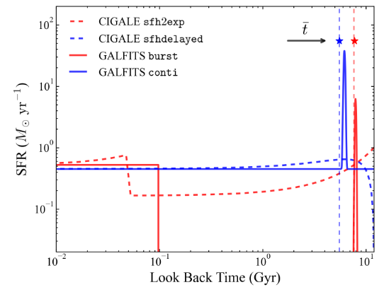
Example of bursty (burst) and continuous SFH (conti) in GalfitS, and their comparison with double exponential (sfh2exp) and delayed tau SFH (sfhdelayed) in CIGALE. The dashed curves represent the sfh2exp (in red) and sfhdelayed (in blue) models, with the vertical dashed line indicating the weighted stellar age (\(\bar{t}\), Equation 19). The parameters for these curves are randomly sampled as in Section 4.1.2. The solid curves show the SFHs recovered by fitting mock photometric data points generated based on the SFHs of the dashed curves, using the burst (red) and conti (blue) models in GalfitS, respectively. This approach demonstrates a good agreement in the shape of the input (dashed curves) and output (solid curves) SFHs. The fitted values of \(\bar{t}\), marked by stars on the graph, also closely match the input values.
Bins SFH
Bins SFH: A more flexible approach where the SFH is divided into discrete time bins, each with a constant SFR. The SFR in each bin is controlled by the 9th parameter (
Pa9), and the ages of the bins are defined by the 10th parameter (Pa10). The bins must be ordered from most recent (first bin, typically at 0 Gyr) to oldest (last bin).
The three SFH types have distinct functional shapes and are controlled by the 9th and 10th parameters. Examples of their configurations are provided below:
For Burst SFH:
Pa9) [[-1,-4,0,0.1,1]]  # contemporary log star formation fraction
Pa10) [[5,0.01,10,0.1,1]]  # burst stellar age [Gyr]
Pa9: Logarithm of the fraction of stellar mass formed in the last 100 Myr.Pa10: Look-back time (age) of the SSP representing the burst.
For Continuous SFH:
Pa9) [[-1,-4,0,0.1,1]]  # contemporary log star formation fraction
Pa10) [[5,0.01,10,0.1,1]]  # burst stellar age [Gyr]
Pa9: Logarithm of the fraction of stellar mass formed since 200 Myr after the Big Bang.Pa10: Age of the SSP burst.
For Bins SFH:
Pa9) [[-2,-8,0,0.1,1],[-2,-8,0,0.1,1],[-2,-8,0,0.1,1],[-2,-8,0,0.1,1],[-1,-8,0,0.1,0]]  # logMass_fraction formed at each time bin
Pa10) [0.,0.1,0.5,1.5,3,13.6]  # age time bins [Gyr]
Pa9: Logarithm of the stellar mass fraction formed in each bin (length: number of bins). The last fraction is typically fixed to avoid degeneracy.Pa10: Look-back ages defining the bin edges (length: number of bins + 1), ranging from 0 Gyr (most recent) to the oldest age (e.g., 13.6 Gyr).
The burst and continuous SFHs provide simpler models with fewer parameters, while the bins SFH offers greater flexibility by allowing the user to define custom time intervals and SFRs for a more detailed reconstruction of the galaxy’s star formation history.
Visualizing SFH Results
After fitting, the SFH can be visualized using the following Python code:
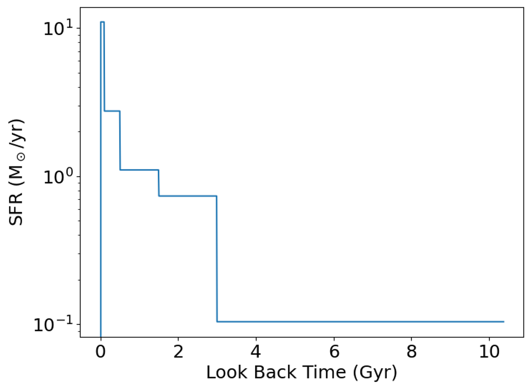
# The galaxy is at z=0.2691, cosmic age about 10.57 Gyr
pltwave, Sedcomp, Sedlabel, z0 = Myfitter.cal_model_image()
modelg = Myfitter.model_list[1]
times, SFHs = modelg.get_SFH()

fig = plt.figure(figsize=(8,6))
plt.plot(times, SFHs[0])
plt.xlabel('Look Back Time (Gyr)', fontsize=18)
plt.ylabel('SFR (M$_\odot$/yr)', fontsize=18)
plt.tick_params(labelsize=18)
plt.yscale('log')
plt.show()
The resulting plot displays the star formation rate (SFR) as a function of look-back time:
Constraining SFH through Priors
The star formation history can be further constrained by setting astrophysical priors in the prior file. These priors impose functional forms on the SFH, such as exponential or delayed-tau models, and are particularly useful for the bins SFH type. Below are examples of how to set priors for different SFH functional forms:
Exponential Increase:
# For exponential increase: SFR(t) = SFR0 * exp((t - t0) / tau)
SFHa1) total
SFHa2) exponential
SFHa3) [[1.,-0.5,2,0.1,1],[0.15,-0.2,0.6,0.1,1],[0.65,0.,1.3,0.1,1]]
SFHa4) [[1.04,0.16],[0.15,0.04],[0.65,0.18]]
Delayed Tau:
# For delayed tau: SFR(t) = SFR0 * (t / tau^2) * exp(-t / tau)
SFHa1) total
SFHa2) delayed
SFHa3) [[1.,-0.5,2,0.1,1],[0.15,-0.2,0.6,0.1,1]]
SFHa4) [[1.04,0.16],[0.15,0.04]]
Double Exponential:
# For double exponential: SFR(t) = SFR0 * (exp((t - t0) / tau0) - k * exp((t - t1) / tau1))
SFHa1) total
SFHa2) exponential2
SFHa3) [[0.4,-0.5,2,0.1,0],[0.15,-0.2,0.6,0.1,1],[0.65,0.,1.3,0.1,1],[0.15,-0.2,0.6,0.1,1],[0.65,0.,1.3,0.1,1]]
SFHa4) [[1],[],[],[],[]]
In this model, the star formation rate (SFR) is modeled as the sum of two exponential components: one representing the older population and one representing a recent burst. The model parameters are given as follows:
logSFR0: The logarithm of the normalization of the SFR.tau0: The exponential timescale for the older population.f: The fraction of the stellar mass coming from the recent burst.tau1: The exponential timescale for the recent burst.t1: The onset time of the recent burst.
The double exponential SFH is defined by
where:
\(t\) is the cosmic time.
\(t_0\) is the age of the Universe (by default, the present time).
The first term models the older stellar population.
The second term models the recent burst.
Here, \(f\) is defined as the fraction of stellar mass formed in the recent burst, and \(k\) is the amplitude scaling the burst contribution in the SFR. To derive the relationship, we integrate each exponential term over time.
By definition \(f\) is the burst stellar mass fraction then by definition
We can solve \(k\) based on \(f\) :
This expression converts the burst stellar mass fraction \(f\) into the amplitude \(k\) for the recent burst term.
These priors are applied only when the SFH type is set to bins in the configuration file. For example:
Pa9) [[0,-8,8,0.1,0],[0,-8,8,0.1,0],[0,-8,8,0.1,0],[0,-8,8,0.1,0],[0,-8,8,0.1,0],[0,-8,8,0.1,0],[0,-8,8,0.1,0],[0,-8,8,0.1,0],[0,-8,8,0.1,0],[0,-8,8,0.1,0],[0,-8,8,0.1,0],[0,-8,8,0.1,0]]  # logMass_fraction formed at each time bin
Pa10) [0.,0.033,0.05681831,0.09782788,0.16843678,0.29000887,0.4993277,0.85972583,1.4802471,2.5486407,4.3881655,7.5553966,13.008631]  # age time bins [Gyr]
...
Pa15) bins
Using more bins improves the resolution of the SFH. An example of a double exponential SFH fit is shown below:
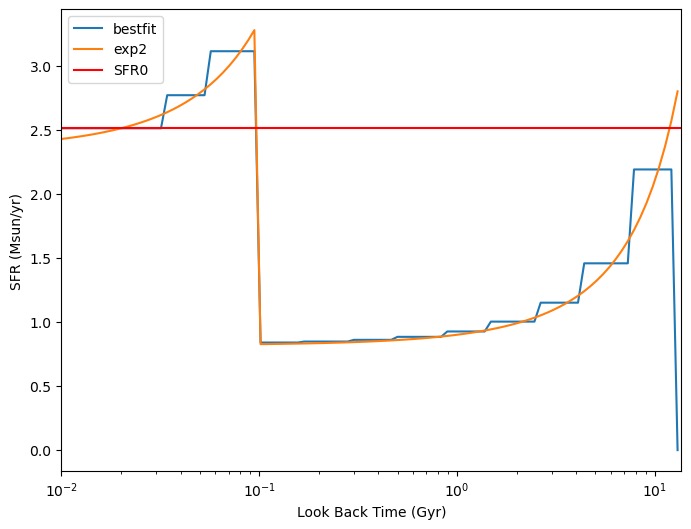
In principle, the normalization parameter (e.g., SFR0) is degenerate with the stellar mass. However, when the prior in SFHa4 has a length greater than zero for the first element (i.e., len(SFHa4)[0] > 0), it incorporates a constraint on the recent SFR, fitting it to a specific value (e.g., the most recent SFR in the above figure).
Run GalfitS on galaxy sample
To run GalfitS on a sample of galaxies, you first need to generate configuration files for each galaxy. These config files specify the parameters and data files for the fitting process. For details on the configuration file format, see config_example.
For instance, if you want to perform SED analysis using the config in SEDfit.lyric, you can use the following Python script to generate config files for all galaxies in your sample:
import os
from astropy.table import Table

# Load the galaxy sample
sample = Table.read('galaxy_sample.txt', format='ascii')
outpath = './configs/'
if not os.path.exists(outpath):
    os.makedirs(outpath)

standard_config = './phot.lyric'
imgpath = '/path/to/your/photometric_data/'
with open(standard_config, 'r') as standard:
    for galaxy in sample:
        name = galaxy['name']
        ra = galaxy['ra']
        dec = galaxy['dec']
        z = galaxy['z']
        outname = os.path.join(outpath, 'SEDfit_2exp.lyric')
        with open(outname, 'w') as fobj:
            for liindex, line in enumerate(standard):
                if liindex == 4:
                    fobj.write("R1) {0}\n".format(name))
                elif liindex == 5:
                    fobj.write("R2) [{0},{1}]\n".format(ra, dec))
                elif liindex == 6:
                    fobj.write("R3) {0}\n".format(z))
                elif liindex == 10:
                    img = imgpath + '{0}'.format(name) + 'band1.fits'
                    fobj.write("Ia1) [{0},0]\n".format(img))
                elif liindex == 12:
                    img = imgpath + '{0}'.format(name) + 'band1.fits'
                    fobj.write("Ia3) [{0},2]\n".format(img))
                elif liindex == 13:
                    img = imgpath + '{0}'.format(name) + 'band1.fits'
                    fobj.write("Ia4) [{0},3]\n".format(img))
                else:
                    fobj.write(line)
            standard.seek(0)  # Reset file pointer for next galaxy
This script reads a standard config file and, for each galaxy in the sample, creates a new config file by modifying specific lines with the galaxy’s name, coordinates (RA and Dec), redshift (z), and paths to the photometric image files. The full script can be found in write_configs.py.
Running GalfitS in Parallel with MPI
Once you have generated the configuration files for all galaxies in your sample, you can run GalfitS on each config file. For large samples, it is efficient to parallelize the fitting using mpi4py. Below is an example script that distributes the config files across available MPI processes:
from astropy.table import Table
from mpi4py import MPI
import subprocess
import os

comm = MPI.COMM_WORLD
rank = comm.Get_rank()
size = comm.Get_size()

sample = Table.read('./gs_test.txt', format='ascii')
loop = rank  # Start from rank to distribute tasks correctly
stop = len(sample)
while loop < stop:
    tagname = sample['ID'][loop]
    dic = './result/{0}/'.format(tagname)
    if not os.path.exists(dic):
        os.makedirs(dic)
    config_file = './configs/SEDfit_2exp.lyric'  # Match config name from generation
    cmd = 'CUDA_VISIBLE_DEVICES={0} python galfitS.py --config {1} --work ./2com --num_s 15000'.format(rank, config_file)
    proc = subprocess.Popen(cmd, shell=True, stdout=subprocess.PIPE, stdin=None, cwd=dic)
    proc.communicate()
    loop += size
To run this script, use the following command:
mpirun -n 4 python galfitS_mpi.py
This command runs the script on 4 processes, each potentially using a different GPU if available, with each process handling a subset of the galaxies in the sample.
If you have a limited number of GPUs, you can modify the script to run on the CPU by removing the CUDA_VISIBLE_DEVICES setting:
cmd = 'python galfitS.py --config {0} --work ./2com --num_s 15000'.format(config_file)
Alternatively, you can specify specific GPU IDs, e.g., CUDA_VISIBLE_DEVICES=0,1,2,3, or set OMP_NUM_THREADS for multi-threading on the CPU. Refer to the GalfitS documentation for detailed instructions on CPU execution.
Note: Ensure that galfitS.py is in your PATH or provide the full path in the command. The options --work ./2com --num_s 15000 are example-specific and should be adjusted according to your requirements.