Quick Start to GalfitS Everything
We will use GalfitS to perform a bulge-disk decomposition of a galaxy J0056-0021, using multi-band images from 10 images from GALEX, SDSS, and 2MASS. The data can be downloaded from data.zip
We will use the configuration file quickstart.lyric to run GalfitS. Let’s first move to the directory where the data is located:
unzip ../../examples/data.zip
cd data
mv ../quickstart.lyric .
Now we can run GalfitS:
galfits quickstart.lyric --work ./result --num_steps 15000
The result will be saved in the directory result. We choose 15000 steps to ensure the result is converged.
Now we can check the result. First, in the directory result, there is a summary file named J0056-0021.gssummary. The first part of the file looks like this:
# target: J0056-0021
# config file: quickstart.lyric
# fitting mode: images - SED
# fiting method: optimizer
# chisq: 14326.755859375
# reduced chisq: 0.5901126861572266
# BIC: 14750.84375
# fitting time: 11.773038339614867 mins
############# data summary ##############
# image atals: 2mass
#    image number: 0  band: j  chisq: [479.75192]  dof: [676.]  reduced chisq: [0.7096922]
#    image number: 1  band: h  chisq: [266.45596]  dof: [676.]  reduced chisq: [0.39416564]
#    image number: 2  band: ks  chisq: [352.4618]  dof: [676.]  reduced chisq: [0.5213932]
# image atals: galex
#    image number: 0  band: galex_fuv  chisq: [235.94382]  dof: [256.]  reduced chisq: [0.92165554]
#    image number: 1  band: galex_nuv  chisq: [550.92737]  dof: [256.]  reduced chisq: [2.15206]
# image atals: sdss
#    image number: 0  band: sloan_u  chisq: [2409.7078]  dof: [4356.]  reduced chisq: [0.5531928]
#    image number: 1  band: sloan_g  chisq: [2535.5747]  dof: [4356.]  reduced chisq: [0.5820879]
#    image number: 2  band: sloan_r  chisq: [2095.2021]  dof: [4356.]  reduced chisq: [0.48099223]
#    image number: 3  band: sloan_i  chisq: [2613.1365]  dof: [4356.]  reduced chisq: [0.59989357]
#    image number: 4  band: sloan_z  chisq: [2787.595]  dof: [4356.]  reduced chisq: [0.6399438]
############ fitting summary ############
This summary provides an overview of the fitting results, including the target name, configuration file, fitting mode, method, chi-square values, reduced chi-square, Bayesian Information Criterion (BIC), and the fitting time. It also includes a detailed breakdown of the chi-square values for each image in the different image atlases (GALEX, SDSS, 2MASS), showing the chi-square, degrees of freedom (dof), and reduced chi-square for each band.
The second part of the file is the summary of the parameters:
pname    best_value
disk_age_value    1.5849
disk_Z_value    0.0300
disk_Av_value    0.4300
logM_disk    10.2398
disk_xcen    -0.5388
disk_ycen    -0.3541
disk_Re    15.0592
disk_ang    -43.6280
disk_axrat    0.4126
bulge_age_value    0.3981
bulge_Z_value    0.0200
bulge_Av_value    1.0165
logM_bulge    10.6108
bulge_xcen    -0.1534
bulge_ycen    -0.1036
bulge_Re    3.1752
bulge_n    4.2031
bulge_ang    24.9169
bulge_axrat    0.7701
......
This table lists the best-fit values for each parameter, such as the age, metallicity (Z), dust extinction (Av), logarithmic stellar mass (logM), star formation history (SFH, see details in Appendix ), and structural parameters (e.g., effective radius Re, position angle ang, axis ratio axrat) for both the disk and bulge components.
The above file can be easily read using astropy.table, for example:
import astropy.table as Table
result = Table.read('result/J0056-0021.gssummary', format='ascii')
logM_bulge = result['best_value'][result['pname'] == 'logM_bulge'][0]
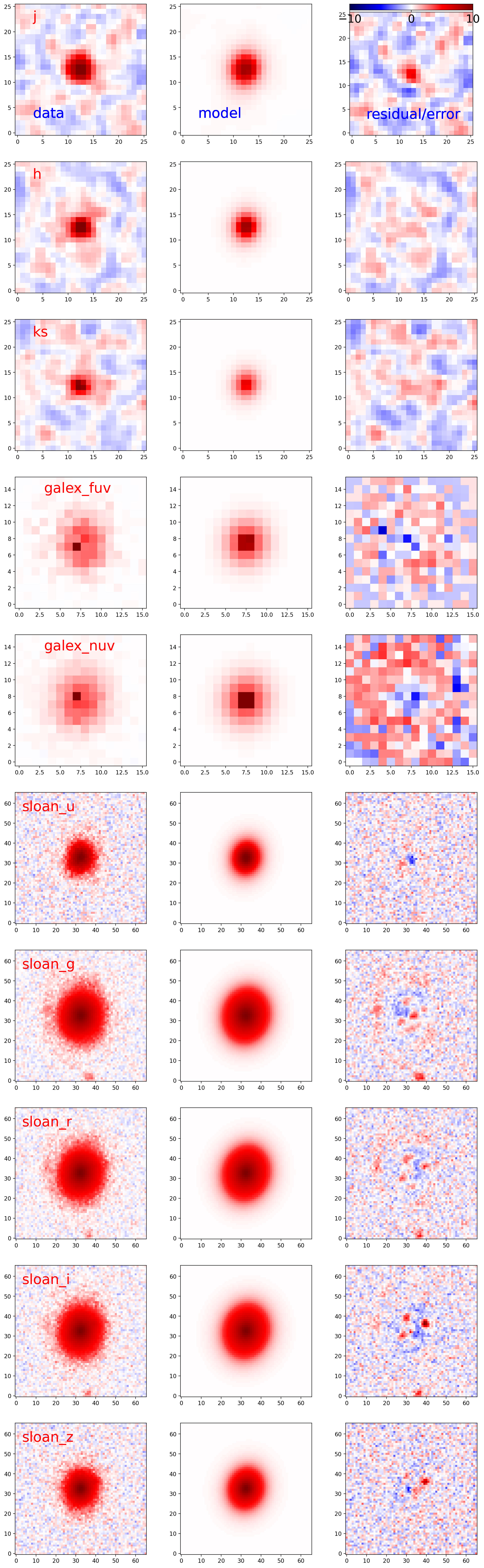
Besides the summary files, there are also two output images. The first is J0056-0021image_fit.png, which displays the original image, the model image, and the residual image for each band:
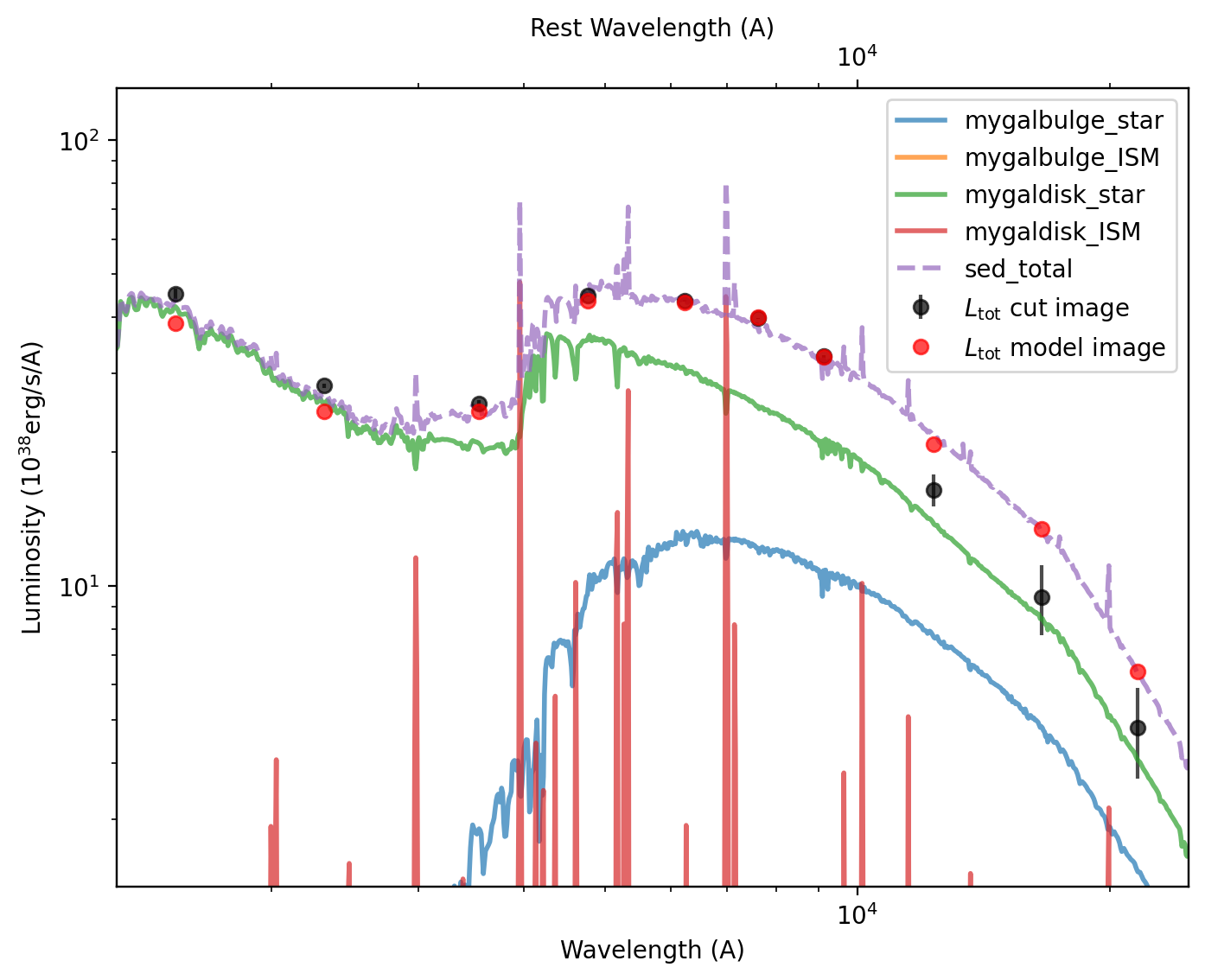
The second output image is J0056-0021SED_model.png, which shows the SED model for the bulge and disk components, along with the model points for each band and a simple photometry measurement:
Running the above example takes different times on different machines. Below is a table summarizing the approximate fitting times:
Machine |
Time |
|---|---|
RTX 4090 |
2.6 mins |
GTX 980Ti |
6.0 mins |
Apple M4 CPU |
12 mins |
Apple intel CPU |
51 mins |