Examples of Config Files

Multi-band imaging decomposition

Performing multi-band imaging decomposition with a simultaneous SED modeling is a fundamental task with GalfitS. We provide a example as the quickstart of GalfitS, see the Quickstart .

Pure mophology fitting: You can also set all the 15th paramter of images to be False, e.g. Ia15) to 0. In this case, only magnitude of each component/band will be fitted. This mode is useful to perform photometry, in this case, you have to set the magnitude zero point, e.g. Ia10), correct,

Pure SED fitting

Photometric SED fitting involves modeling the SED of an astronomical object using a set of data points derived from broad-band photometry. In GalfitS, this process begins by transforming photometric data into ‘mock’ images, followed by the standard fitting routine. The photometric data is typically provided in a table format, including columns for the band, flux, and flux error. Here’s an example:

Band	Flux	Flux_err
NUV	xxx	xxx
FUV	xxx	xxx
…	…	…

Transforming Photometry Data to Mock Images

To convert this photometric data into mock images, you can use the photometry_to_img function from the galfits.gsutils module. Below is an example Python script to perform this transformation:

from galfits import gsutils
object_flux = Table.read('./object.mag', format='ascii')
z = object['redshift']
Bands = ['galex_nuv', 'galex_fuv', 'sloan_u', 'sloan_g', 'sloan_r', 'sloan_i', 'sloan_z', 'wise_ch1', 'wise_ch2', 'wise_ch3', 'wise_ch4']
for loop, band in enumerate(Bands):
    flux_mjy = object_flux[band]
    flux_err = object_flux[band + '_err']
    outputname = './data/' + band + '.fits'
    gsutils.photometry_to_img(band, flux_mjy, flux_err, z, outputname, unit='mJy')

This script generates a set of mock images, one for each photometric band, which are then used in the SED fitting process.

Configuration File for SED Fitting

An example configuration file for performing SED fitting from the far-ultraviolet (FUV) to the far-infrared (FIR) is available at SEDfit.lyric. In this setup, each photometric data point is treated as an image. Below is an excerpt showing how to configure a photometric data point:

# Image A
Ia1) [/home/liruancun/Works/liyang/cutimgs/photometry/2sloan_u.fits,0]
Ia2) sloan_u      # band
Ia3) [/home/liruancun/Works/liyang/cutimgs/photometry/2sloan_u.fits,2]
Ia4) [/home/liruancun/Works/liyang/cutimgs/photometry/2sloan_u.fits,3]
Ia5) 1                   # PSF fine sampling factor relative to data
Ia6) [Noimg,0]
Ia7) cR                # unit of the image
Ia8) -1
Ia9) 1                # Conversion from image unit to flambda, -1 for default
Ia10) 28.3291              # Magnitude photometric zeropoint
Ia11) uniform             # sky model
Ia12) [[0,-0.5,0.5,0.1,0]]                   # sky parameter, (value, min, max, step)
Ia13) 0                     # allow relative shifting
Ia14) [[0,-5,5,0.1,0],[0,-5,5,0.1,0]] # [shiftx, shifty]
Ia15) 1 # Use SED information

Important Notes:

• The Ia8) parameter is set to -1, indicating that the image size is not used in the conventional sense, as this is a mock image for SED fitting.

• The Ia9) parameter is set to 1, which is essential for converting image units to flux density units (flambda). Using -1 would apply the default conversion, but specifying 1 ensures the correct transformation for SED fitting.

Fitting Results

Once the fitting process is complete, the results are saved in a summary file, accompanied by a figure illustrating the SED fitting outcome. The figure below displays the contributions from different components: stars (blue), nebular emission (green), and dust (red).

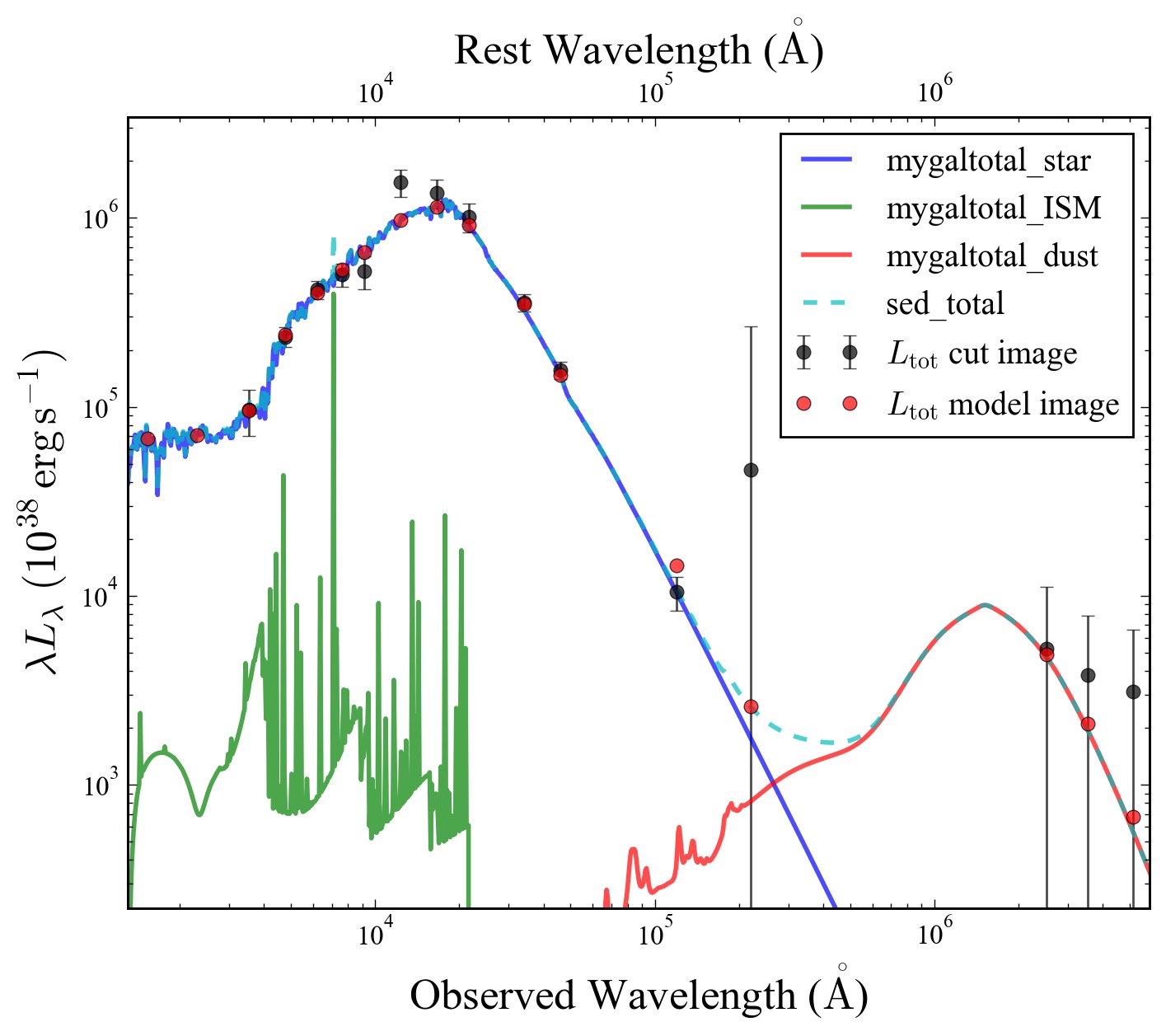
Example of SED fitting results, showing contributions from stars (blue), nebular emission (green), and dust (red).

Performance

The time required to run this SED fitting example varies depending on the machine. Below is a table summarizing approximate fitting times:

Machine	Time
RTX 4090	1.5 mins

Spectrum fitting

To perform spectrum-only fitting in GalfitS, the input spectrum is typically provided as a table without a header. The first column represents the wavelength in angstroms (Å), the second column is the flux (\(F_\lambda\)), and the third column is the flux error. An example snippet of such data might look like this:

3000  xxx  xxx

An example dataset of an AGN spectrum is available at GreeneHo2004_id2.txt.

We will use an example of AGN spectrum decomposition to illustrate the functionality of GalfitS. The example configuration file is AGNspectrum.lyric.

Configuration for Spectrum Input

In the config file for spectrum fitting, spatial parameters like R2) and R3) (region information) become irrelevant and do not need to be configured. To input a spectrum, the following section is used:

# Spectrum
Sa1) GreeneHo2004_id2.txt                  # spectrum file
Sa2) 1                                     # conversion from spectrum unit to 1e-17 flambda
Sa3) [3600., 7000.]                        # wavelength range
Sa4) 0                                     # use high resolution stellar template

# Image atlas
Ab1) sdss                                  # name of the image atlas
Ab2) []                                    # images in this atlas
Ab3) 1                                     # whether the images have same pixel size
Ab4) 1                                     # link relative shiftings
Ab5) ['a']                                 # spectra
Ab6) [[2]]                                 # aperture size
Ab7) [-1]                                  # references images

Here, the spectrum is integrated into an image atlas class via Ab5). Key notes:

• Sa2): Specifies the conversion factor from the spectrum’s native unit to \(10^{-17} F_\lambda\). Adjust this based on your data’s units.

• Sa3): Defines the wavelength range for fitting in the rest frame (e.g., 3600–7000 Å).

• Sa4): Determines the resolution of the stellar template. The default resolution is 150 km/s (Sa4) 0). To measure velocity dispersion accurately, set Sa4) 1 to use a high-resolution template (30 km/s).

• Ab6): Specifies the aperture size. Since this is a single spectrum, no reference image is needed for slit/filter geometry (Ab7) -1).

Model Parameters

In AGNspectrum.lyric, geometric parameters for the host galaxy (e.g., Pa3)-Pa8)) and AGN (e.g., Na4)-Na5)) are not relevant for spectrum-only fitting. Below are some key parameters for the host galaxy and AGN:

Pa9) [[-2,-4,0,0.1,1]]                    # contemporary log star formation fraction
Pa10) [[5,0.01,11,0.1,1]]                 # burst stellar age [Gyr]
Pa11) [[0.02,0.001,0.04,0.001,0]]         # metallicity [Z=0.02=Solar]
Pa12) [[0.7,0.3,5.1,0.1,1]]              # Av dust extinction [mag]
Pa13) [100,40,300,1,0]                    # stellar velocity dispersion
Pa14) [10.14,8.5,12,0.1,1]                # log stellar mass
Pa15) conti                                # star formation history type: burst/conti
...
Na10) [43,41,47,0.1,1]                    # log L5100
Na11) [[1,0,4,0.1,1], [0.6, 0, 5, 0.1,0]] # power law indexes
Na12) ['Hg','Hb','HeII_4686','Ha']        # broad emission lines
Na13) ['Hg','Hb','HeII_4686','OIII_4959','OIII_5007','HeI','Ha','OI_6302','NII_6549','NII_6583','SII_6716','SII_6731'] # narrow emission lines
Na14) 2                                    # number of components for broad lines
Na15) 2                                    # number of components for narrow lines
Na16) 0                                    # add Balmer continuum
Na17) 1                                    # add FeII
Na18) 0                                    # continuum model, 0: power law, 1: broken power law, 2: thin disk

For the host galaxy, we use a continuous star formation history (Pa15) conti), parameterized by the contemporary log star formation fraction (Pa9)) and the burst stellar age (Pa10)). To study velocity dispersion, set Pa13) to be free (last value = 1). For the AGN, we adopt a single power-law continuum model (Na18) 0), include FeII pseudo-continuum (Na17) 1), and exclude the Balmer continuum (Na16) 0) due to wavelength coverage. The broad (Na12)) and narrow (Na13)) emission lines must match definitions in emission_lines.py. Adjust Na14) and Na15) to change the number of components.

Running the Example

Run the fitting with:

galfits ./AGNspectrum.lyric --work ./result/ --num_s 20000

The result includes a figure:

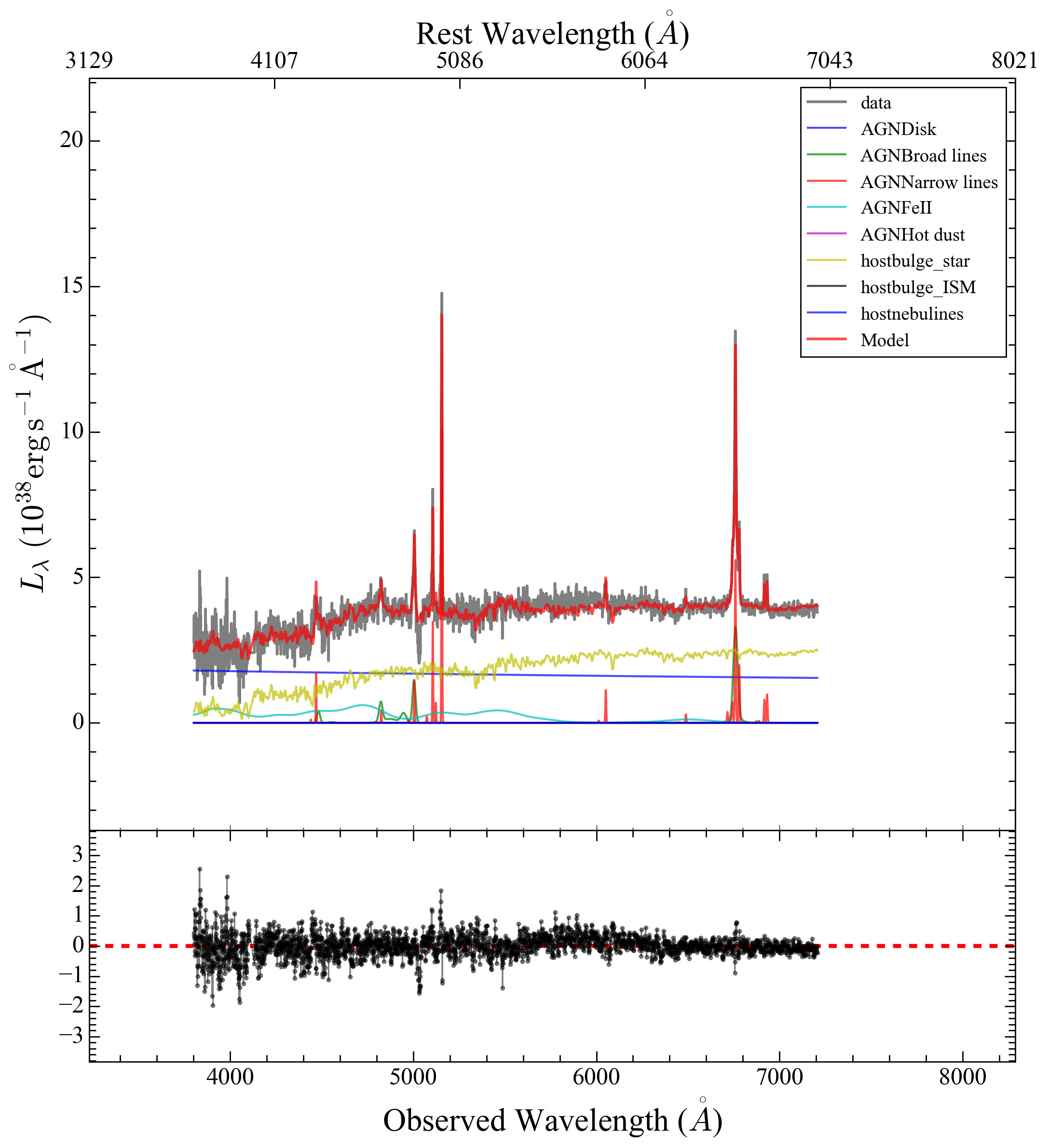
Example of spectrum fitting, where all subcomponents are labeled, and the bottom panel shows the residual.

Manipulating Parameter Files

After running, a parameter file (e.g., J0249-0815.params) is generated in the result folder. You can modify it to refine the fit. Examples:

1. Adjusting Hβ Broad Line Central Wavelength:

   HbAGNb1wid 17.220163213245794 8.265678342357983 82.65678342357981 0.1 True None
   HbAGNb1peak 9975.021484375 0.0 99750.21875 99.75021362304688 True None
   HbAGNb1cen 4862.68 4812.68 4912.68 0.1 True None
   HbAGNb2wid 34.44032642649159 13.776130570596637 82.65678342357981 0.1 True None
   HbAGNb2peak 997.5021362304688 0.0 99750.21875 99.75021362304688 True None
   HbAGNb2cen 4862.68 4762.68 4962.68 0.1 True None
   HbAGNb3wid 34.44032642649159 13.776130570596637 82.65678342357981 0.1 True None
   HbAGNb3peak 997.5021362304688 0.0 99750.21875 99.75021362304688 True None
   HbAGNb3cen 4862.68 4762.68 4962.68 0.1 True None
   

   Here, the initial value and range of the central wavelength (HbAGNb2cen, HbAGNb3cen) for the 2nd and 3rd broad Hβ components are adjusted to 4762.68–4962.68 Å.

2. Reducing HeII Broad Components:

   HeII_4686AGNb1wid 16.598100097836443 7.967088046961493 79.67088046961493 0.1 True None
   HeII_4686AGNb1peak 5994.80859375 0.0 59948.0859375 59.94808578491211 True None
   HeII_4686AGNb1cen 4687.02 4637.02 4737.02 0.1 True None
   HeII_4686AGNb2wid 33.19620019567289 13.278480078269151 79.67088046961493 0.1 False None
   HeII_4686AGNb2peak 0.0 0.0 59948.0859375 59.94808578491211 False None
   HeII_4686AGNb2cen 4687.02 4487.02 4887.02 0.1 False None
   HeII_4686AGNb3wid 33.19620019567289 13.278480078269151 79.67088046961493 0.1 False None
   HeII_4686AGNb3peak 0.0 0.0 59948.0859375 59.94808578491211 False None
   HeII_4686AGNb3cen 4687.02 4487.02 4887.02 0.1 False None
   

   This reduces the HeII fit to one broad component by setting the 2nd and 3rd components’ peak to 0 and fixing their parameters (False).

3. Adding Broad Wings to OIII:

   OIII_4959AGNb1wid 17.56584629995127 8.431606223976612 84.31606223976611 0.1 False 0.990426571*OIII_5007AGNb1wid
   OIII_4959AGNb1peak 1000.0 0.0 1725463.875 172.54638671875 False 0.33557*OIII_5007AGNb1peak
   OIII_4959AGNb1cen 4950.295 4910.295 5010.295 0.1 False 0.990426571*OIII_5007AGNb1cen
   OIII_4959AGNb2wid 35.13169259990254 14.052677039961017 84.31606223976611 0.1 False None
   OIII_4959AGNb2peak 0.0 0.0 93883.40625 93.88340759277344 False None
   OIII_4959AGNb2cen 4960.295 4760.295 5160.295 0.1 False None
   OIII_4959AGNb3wid 35.13169259990254 14.052677039961017 84.31606223976611 0.1 False None
   OIII_4959AGNb3peak 0.0 0.0 93883.40625 93.88340759277344 False None
   OIII_4959AGNb3cen 4960.295 4760.295 5160.295 0.1 False None
   OIII_5007AGNb1wid 17.73563348011922 1.418 85.13104070457226 0.1 True None
   OIII_5007AGNb1peak 3000.0 0.0 172546.390625 172.54638671875 True None
   OIII_5007AGNb1cen 5000.0 4958.24 5058.24 0.1 True None
   OIII_5007AGNb2wid 35.47126696023844 14.188506784095374 85.13104070457226 0.1 False None
   OIII_5007AGNb2peak 0.0 0.0 172546.390625 172.54638671875 False None
   OIII_5007AGNb2cen 5008.24 4808.24 5208.24 0.1 False None
   OIII_5007AGNb3wid 35.47126696023844 14.188506784095374 85.13104070457226 0.1 False None
   OIII_5007AGNb3peak 0.0 0.0 172546.390625 172.54638671875 False None
   OIII_5007AGNb3cen 5008.24 4808.24 5208.24 0.1 False None
   

   This adds a broad wing to OIII, linking OIII_4959AGNb1 to OIII_5007AGNb1 (width, peak, and center) while shutting down the other two components.

After refining the parameters, you can rerun the fitting with the modified parameter file: .. code-block:: bash

galfits ./AGNspectrum.lyric –work ./newresult/ –num_s 20000 –readpar J0249-0815.params

Performance

The time required to run this spectrum fitting example varies by machine:

Machine	Time
RTX 4090	0.5 mins

Imaging + spectrum fitting

Grism imaging fitting